###What is the assignment?
I recently did some analyses of crime rates in San Francisco using their Open Data datasets. This was part of two different assignments for the University of Washington’s “Data Science at Scale” course. One assignment was to use visualization to develop some new inference - I used an iPython / Jupyter notebook that can be found at this link. The second assignment was to compete in a Kaggle competition. My detailed write-up can be found here.
###What did I learn?
I did the exploratory exercise first, and the Kaggle exercise second. Using what I had learned from the exploratory exercise, I began creating new fields before even developing a model. I thought I had information that had explanatory power and that I already knew the solution. This was a huge mistake! I should have started with the dataset and let it give me a sense of what data was valuable and the overall structure. For example, using a cor() plot and/or pulling a variable importance (VarImp() ) from a Random Forest model. Not doing this led to several hours of wasted time and effort.
Running through this exercise had me thinking about the Unreasonable Effectiveness of Data:
“Choose a representation that can use unsupervised learning on unlabeled data, which is so much more plentiful than labeled data. Represent all the data with a nonparametric model rather than trying to summarize it with a parametric model, because with very large data sources, the data holds a lot of detail.
For those with experience in small-scale machine learning who are worried about the curse of dimensionality and overfitting of models to data, note that all the experimental evidence from the last decade suggests that throwing away rare events is almost always a bad idea, because much Web data consists of individually rare but collectively frequent events.“
This is useful when trying to develop the most accurate, dynamic model. But what if I am just trying to learn what is present in the data, and only want a semi-accurate high-level understanding? I had this conversation with one of our Principal Data Scientists, Drew Hardin. His guidance was to, in those situations, throw away as much data as possible. Why run a model on a sample of 700K if a 10K set is just as representative of the population? At the same time (and similar to the Halevy paper), don’t necessarily imbue assumptions of the underlying structure of the data because you made them elsewhere.
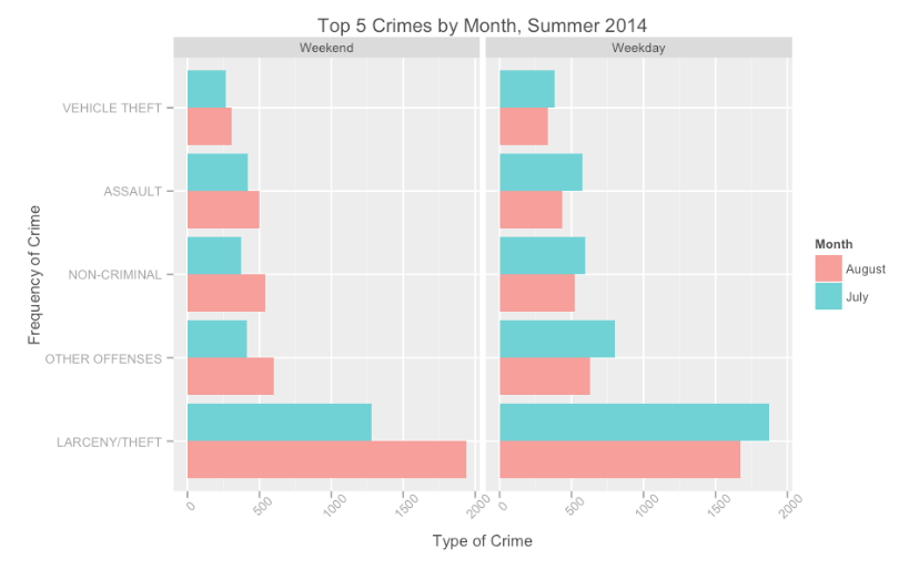
###Exploration Theft/Larceny is by far the most reported crime in the city. After analyzing at reported crimes by day and month, contrary to expectation, I found that July had more crimes reported “midweek” than over the weekends. I peeled into the type of crimes being addressed and found that “Warrants” and “Non-Criminal” activities rise during the week - during weekdays, the police are performing work that can be predicted in advance and managed.
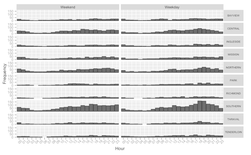
I then looked at different neighborhoods/police districts to see if any patterns might emerge. The city center (SoMA = Southern, Financial District = Central, Tenderloin, etc) is where the highest crime emerges. Peculiarly, weekday crimes have a bump around 12pm and then again between 5-7pm. Presumably, this is when victims realize that a theft has occurred and contact the police. No such pattern is present on the weekends.
Looking here, we can see that July’s pattern of increased reporting during weekdays holds true across the board. There are, on average, almost 50% higher reporting of theft on weekdays than weekends - a trend that is not true for the month of August.

My conclusion is that over the weekend, people are not in town to report crimes. The elevated numbers are not due to the distribution of when the events occurred, but rather when they were reported.
Let’s now look at the Police Departments in San Francisco and where crimes are reported. The Top 4 (by volume of crime) are Central, Northern, Southern, and Mission. This would be expected, as they are in the city center and cover a relatively large volume of the city. The Tenderloin (#7) is known for not being safe, but is comparatively small.

###Kaggle Competition
The task is to predict the category of of a crime in San Francisco based on a variety of attributes, including the time at which the crime was reported, the street address, the day of the week, a general description of the crime, the precint reporting, and Lat/Long information. We are given the last 12 years of information, from 2003-2015, which provides ~878K reports.
There are 39 different different classes in the category we are trying to predict, although they are certainly not distributed evenly. The top 3 are “Larceny/Theft”, “Other Offenses”, and “Non-Criminal” with ~175K, ~125K, and ~92K reports, respectively. Solutions are evaluated by comparing the percentage of correct answers on a test dataset. The actual scoring is based “log loss.” It takes the probability of being able to predict the correct answer and uses the equation “LN(P(x)) - 1”.
Not seeing a good way to take the text data from “Address” and seeing that the precincts are too large to offer predictive value, I used the Lat/Long information to bin the different crimes. I dropped the ~700 values that did not have Lat/Long info (marked as -120.5, -90), and originally split the rest into a 100x100 grid. However, the bins were too small, some having only ~100 crimes. I reestablished the bins for a 25x25 grid (625 bins for SF).
Originally, I wanted to run a RandomForest model against all features and have the model tell me the variable importance of the different features (using the varImp() function). However, I ran into quite a few snags before making a submission.
- First, randomForest in R does not take NAs. It has a few options for addressing this in ‘na.action’, but I wasn’t sure if there was information I might have been leaving out by imputing the NAs.
- Second, randomForest in R only takes features with 53 or fewer bins. Therefore, my location bucketing (625 bins) was not acceptable. I split them into Lat and Long variables separately and hoped that the interaction would be picked up in the model.
- The randomForest challenges led me to try R’s other decision trees package, rpart(). However, the dataset was too large to get the algorithm to converge. I tried several things, none of which worked:
- I adjusted the sample size from ~878K down to 10K using the sample() function,
- I adjusted the minimum bucket size to 100 samples to reduce the number of splits in the model,
- I adjusted the complexity parameter to 0.01 to adjust when the model would accept a split as being necessary, and
- I took the 39 classes in the predictor and reduced it to 5 for model simplicity. In this final state, I let R run for ~4 hours and decided for a different approach when it did not converge.
- To get a convergence, I went back to the randomForest() model and decided to drop all rows that have an “NA” present. I also used the 10K sample instead of the full ~878K set
- Finally, running the model against the test set results in a list of ~885K predictions. Kaggle asks for the submission to be a sparse matrix of 1s and 0s (with the different classes as the column headings). I wrote a nested for loop to make this conversion, which isn’t great for R’s memory capabilities. That is - it starts off fast, and then slows as the matrix builds. I switched to the lapply() and my speeds dropped considerably.
- There seem to be two poles to the submissions - the first thousand submissions and the second thousand submissions have very different predictive capabilities. Reading through some answers, I realized the fields that I added were what gave me poor predictive information. If I ran randomForest without the extra fields, that would have put me in the top bucket of answers.
Now, if I had tried to place in the top ~25 spots - that would have required the Unreasonable Effectiveness of Data approach: I read through the open scripts for a few of the top answers, which use a combination of Keras, a deep learning library for Theano or TensorFlow, and a count featurizer from Microsoft Azure, which uses the frequency of events to indicate the strength or importance of different given features.
